Gradient Descent
The core loop Training a model means finding the settings of its knobs, the weights, that make its errors as small as possible. The error as a function of the weights forms a surface in a high-dimens
Oct 13, 2026 · 4 min read
The core loop
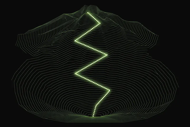
Training a model means finding the settings of its knobs, the weights, that make its errors as small as possible. The error as a function of the weights forms a surface in a high-dimensional space: every combination of weights has a height equal to how wrong the model is with those weights. Training is the search for the lowest point on that surface.
Gradient descent is the workhorse algorithm for that search. At the current position, compute the gradient: the direction in which the error rises most steeply. Then take a step in the opposite direction. Repeat. The update rule for each weight is:
```
w = w - learning_rate * (dL/dw)
```
The gradient points uphill, so stepping against it goes downhill. The learning rate controls the step size. That is the whole algorithm. Everything else in optimization is a refinement of this loop.
A minimal example makes it concrete. Here is gradient descent minimizing a simple parabola, where the answer should be x = 3:
```python
def loss(x):
return (x - 3) ** 2
def gradient(x):
return 2 * (x - 3)
x = 0.0
learning_rate = 0.1
for _ in range(50):
x = x - learning_rate * gradient(x)
print(x) # converges toward 3.0
```
A neural network does the same thing with millions of weights at once, using backpropagation to compute all the gradients efficiently.
The learning rate
The learning rate is the single most consequential setting in training. Too large, and the steps overshoot: the error bounces around or explodes to infinity. Too small, and training crawls, wasting compute and risking getting stuck in a mediocre spot.
In practice the learning rate usually changes during training. A common schedule warms it up from near zero, holds it steady while the model learns the broad structure, then decays it so the final steps settle precisely into place. Cosine decay, which lowers the rate along a smooth curve to near zero, is a popular choice. Getting this schedule right matters as much as picking the architecture.
Batch, stochastic, and mini-batch
The gradient can be computed over different amounts of data. Full-batch gradient descent uses the entire dataset for each step, giving the true downhill direction but requiring a full pass over the data per update, which is impractical at scale. Stochastic gradient descent uses a single example per step: each step is noisy, but steps are cheap and the noise can actually help escape shallow traps. Mini-batch gradient descent splits the difference, computing the gradient over a few dozen to a few thousand examples. Nearly all neural network training uses mini-batches, because they parallelize well on GPUs while keeping the gradient estimate stable enough.
The idea of using noisy gradient estimates for optimization goes back to Robbins and Monro's 1951 work on stochastic approximation. The method of steepest descent itself is older still, introduced by Cauchy in 1847.
Beyond vanilla: momentum and Adam
Plain gradient descent struggles on surfaces with long narrow valleys: it oscillates across the valley while creeping along it. Momentum fixes this by giving the update a velocity that accumulates across steps. Oscillations cancel out while consistent downhill directions build up speed, like a ball rolling downhill gaining momentum.
Adam, introduced by Kingma and Ba in 2014, is the default optimizer for most deep learning. It keeps two running averages per weight: one of the gradients (like momentum) and one of the squared gradients (measuring how noisy each weight's signal is). Each weight's step is then scaled by its own noise level, so weights with steady signals take confident steps while weights with erratic signals step cautiously. AdamW, a variant that handles weight decay correctly, is the standard for training transformers.
These adaptive methods converge faster and need less tuning than plain gradient descent, which is why they dominate in practice. They are not magic: on some problems, carefully tuned plain SGD with momentum still generalizes slightly better.
Local minima and saddle points
A persistent worry is that gradient descent will get stuck in a bad local minimum, a valley that is not the deepest one. In the high-dimensional spaces of neural networks, this turns out to be less of a problem than feared. True local minima are rare in very high dimensions; what look like traps are usually saddle points, flat in some directions and sloping in others. Gradient descent with a little noise tends to slide off saddles eventually, which is one reason the stochasticity of mini-batch training helps rather than hurts.
The deeper truth is that for overparameterized networks, most minima the optimizer finds are about equally good. The goal is not the global optimum, which is unfindable and unnecessary, but any of the many valleys where the model generalizes well.
What can go wrong
Two failure modes deserve mention. Vanishing gradients happen when the gradient shrinks as it travels back through many layers, leaving early layers essentially untrained. This plagued deep networks until ReLU activations and better initialization tamed it. Exploding gradients are the opposite: the signal grows until the weights blow up to infinity. Gradient clipping, which caps the gradient's size before applying the update, is the standard fix and is routine in training language models.
Comments
Loading comments…